Case Study: Linear Regression & Business Decision Making

Introduction

This paper will examine a case study presented by Esö et al. (2017) in “Pedigree vs. Grit: Predicting Mutual Fund Manager Performance”. The case study uses linear regression to evaluate fund manager performance based on five independent variables (Esö et al., 2017). More specifically, there are two candidates, Bob and Putney, being considered for an important role that come from different backgrounds (Esö et al., 2017). An analysis is done on the industry to prove empirically whether certain qualities and experiences have an impact on excess returns generated (Esö et al., 2017).

R-Squared

One of the main premises of the case is that linear regression results are being disregarded as “useless” by the CEO, Jack, due to the low R-squared value (Esö et al., 2017). The full output of this regression analysis can be seen in Figure 1. As can be seen, the R-squared value is only 4.33% (Esö et al., 2017); however, this does not necessarily mean that the results are useless, as the R-squared value simply represents the amount of variability that can be explained by the model (French, 2023).

A low R-squared value might tell you two important things: some variance is explained by the constructed model, and there are other influential factors that are not being considered. In contrast, results with high R-squared values may not automatically be considered useful. For example, variables may have high levels of multicollinearity, making it difficult to determine the true effect size of each independent variable (Princeton DSS, 2007).

Other assumptions should be checked for linear regression models, such as the model presented in this case. Some assumptions, such as linearity, can often be validated visually (French, 2022). Homoscedasticity, which is the assumption that all residuals have equal variance, can sometimes be validated visually as well (Struck, 2024). Statistical tests, such as the Breusch-Pagan test, may also be used to validate this assumption (Struck, 2024).

Model Estimates

The case study continues under the premise that Jack is then convinced that the regression analysis may have some usefulness despite the low R-squared value (Esö et al., 2017). He proceeds to ask a series of questions about what the model predicts (Esö et al., 2017).

First, he wants to predict the excess returns that would be generated by Bob and Putney at their current funds using the model parameters, known information about the candidates, and average SAT scores from their alma maters (Esö et al., 2017). It can be estimated that Bob would generate an estimated excess return of -1.78% while Putney would generate an estimated excess return of 0.40%. This results in an estimated 2.18% spread in Putney’s favor.

Jack requests a similar analysis to be performed, except this time he wants to know what the estimated excess return would be if Bob and Putney were hired to manage a new fund (Esö et al., 2017). The only variable that would change in this case is tenure would be set to zero for both candidates, resulting in an estimate of -1.19% for Bob and 0.63% for Putney. This ends up being an estimated 1.82% spread in Putney’s favor.

Jack then asks if you could “prove at the 5 percent significance level that if Bob had attended Princeton instead of Ohio State, then the return of his current fund would be greater” (Esö et al., 2017, p. 4). The answer to this question is “yes and no”. The alma mater of the candidate is not directly represented in the model; however, since Jack is using the schools as a proxy for SAT scores, it is relevant to the question. Furthermore, SAT score as an independent variable is statistically significant at the 5% significance level and has a positive correlation with excess returns.

The next question Jack has is if “you [can] prove at the 10 percent level of significance that if Bob were managing a growth fund instead of a growth and income fund, then he would achieve at least 1 percent higher average returns” (Esö et al., 2017, p. 4). The answer to this question is a clear “yes”; however, it is applicable to both candidates. GRI is a “dummy variable that equals one if Morningstar classifies this fund as a growth and income fund, and zero if it is classified as simply a growth fund” (Esö et al., 2017, p. 3). The coefficient is -2.11046 (Esö et al., 2017), suggesting that both candidates would achieve an additional ~2.11 percentage points in excess returns if they were running growth funds rather than growth and income funds. Not only is this variable statistically significant at the 10% level, but it is also the most significant independent variable, with a p-value of just 0.4452% (Esö et al., 2017).

In contrast, “MBA” is the independent variable with the weakest level of statistical significance, having a p-value of 81.139% (Esö et al., 2017). This does not add much supporting evidence for the idea that having an MBA has an impact on fund performance. The claim made by some is “that fund managers without MBAs get higher expected returns because they invest in riskier stocks” (Esö et al., 2017, p. 4). If this claim were true, one might be able to include Beta as an additional independent variable in the model to isolate general appetite for risk from other factors that might be associated with a manager having an MBA. This additional variable would likely reduce the magnitude of the MBA coefficient if the assumption were true. It would also be important to check for multicollinearity between the MBA variable and Beta.

Jack then wants to know “the lowest level of significance at which you can prove that the manager’s age has a negative impact on his or her fund’s performance holding the type of the fund, the manager’s education, and years of experience at the fund constant” (Esö et al., 2017, p. 4). Since the age variable has a p-value of 10.006% (Esö et al., 2017), this is the lowest level of significance at which the relationship can be proven. It’s also noted that survivorship bias has an impact on the age variable since “a younger manager’s survival in the industry is more closely linked to his/her performance than an older manager’s survival” (Esö et al., 2017, p. 4). This bias likely skews the coefficient in favor of younger managers.

After eliminating all variables that are not statistically significant at least at the 15% level, the remaining equation is RET = -2.11046(GRI) + 0.005735(SAT) - 0.068893(AGE) + Constant, where the constant is equal to -2.64216; however, Jack is informed that the regression analysis needs to be rerun, including only these parameters, as the values will change when the additional variables are excluded. Interactions between variables may have an effect on the magnitude and/or direction of the remaining coefficients.

Jack continues to focus on the SAT variable as a proxy for alma mater. He understands that a new regression analysis would need to be executed if nonsignificant variables were to be accurately excluded from the model; however, he wants to use the current model to better understand the mechanics of linear regression.

First, Jack wants to know how a new fund with a Princeton alumnus (same alma mater as Putney) would perform (Esö et al., 2017). If all other unknown variables were set equal to Putney’s variables, it could be expected that the fund would generate an excess return of ~0.63%, the same as would be expected of Putney if she had zero tenure. Jack wants to know how confident he could be in this analysis that a fund manager with this profile would truly beat the market (yield excess returns greater than zero) (Esö et al., 2017). To answer this question, the “standard error of the regression” (SER) can be used. This statistic can be used to assess the amount of noise that exists within a given dataset (Nau, 2020). The SER of 8.354658 (Esö et al., 2017) can be multiplied by the T-statistic for computing 95% confidence intervals for this model, which is 1.9644 (Esö et al., 2017), resulting in ~16.41. This number can then be added and subtracted from the estimated excess returns to construct a confidence interval of [-15.78, 17.04]. Based on this interval, it would be fair to have hesitancy about this model proving that a candidate with this profile would truly generate excess returns.

Jack wonders what the model would say if he identified a large number of funds with similar profiles and invested equally in all of them (Esö et al., 2017). The law of large numbers (LLN) explains that as the number of observations increases, their average value will begin to converge to the average of the population (Law of Large Numbers, n.d.). Based on this fact alone (and assuming the current model is sufficient), there is not enough information to assume that increasing the sample size would result in excess returns that vary dramatically from those predicted by the model.

Conclusion

Based on the results of this preliminary regression model alone, it would make sense to recommend Putney for the job over Bob. While the predictive power of the model is dubious, it does show that certain variables do have at least some correlation with fund performance. Each of these indications is favorable for Putney.

References

Esö, P., Hunter, G., Klibanoff, P., & Schmedders, K. (2017). Pedigree vs. Grit: Predicting Mutual Fund Manager Performance. Kellogg School of Management Cases, 1–6. https://doi.org/10.1108/case.kellogg.2016.000257

French, T. (2022, September 11). Visualizing OLS linear regression assumptions in R. Medium. https://medium.com/trevor-french/visualizing-ols-linear-regression-assumptions-in-r-e762ba7afaff

French, T. (2023). R for Data Analysis: An open-source resource for teaching and learning analytics with R. Journal of Open Source Education, 6(63), 202. https://doi.org/10.21105/jose.00202

Law of large numbers. (n.d.). Encyclopedia of Mathematics. Retrieved July 20, 2025, from http://encyclopediaofmath.org/index.php?title=Law_of_large_numbers&oldid=55010

Nau, R. (2020). Linear regression models. Duke University. Retrieved July 20, 2025, from https://people.duke.edu/~rnau/regnotes.htm

Princeton DSS. (2007). DSS - Interpreting Regression Output. Princeton University. Retrieved July 19, 2025, from https://dss.princeton.edu/online_help/analysis/interpreting_regression.htm

Struck, J. (2024, June). Regression Diagnostics with R. University of Wisconsin Social Science Computing Cooperative. Retrieved July 19, 2025, from https://sscc.wisc.edu/sscc/pubs/RegDiag-R/index.html

Appendix

Figure 1 Regression table from the case study 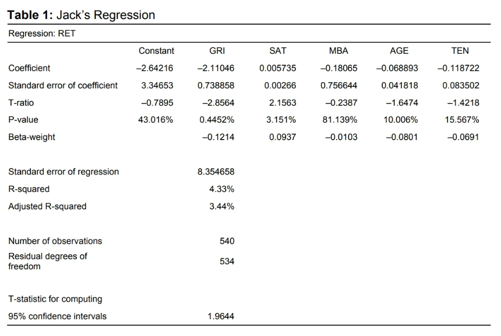Note. Image retrieved from “Pedigree vs. Grit: Predicting Mutual Fund Manager Performance” by Esö et al. (2017)